10. Lecture #10

We learned about ordinary differential equations, and how to integrate them numerically.

Scribe Notes by Monica Giragosian: PDF1

Scribe Notes by Tavel Findlater: Source2 PDF2

Numerical Integration

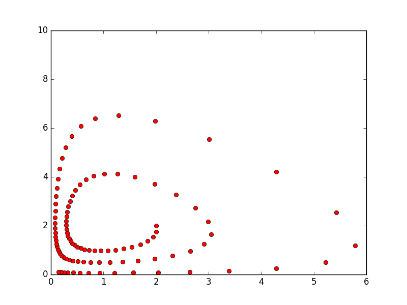
The Lotka-Volterra model for the predator-prey problem comprises of the following system of ordinary differential equations

\[\begin{split}\dot{u} = u(v-2) \\ \dot{v} = v(1-u)\end{split}\]

Python code for a forward Euler discretization of the above system with a time step size of \(\Delta t = 0.12\) is given below, and generates the plot shown above.

import matplotlib.pyplot as plt

u = [2]
v = [2]
h = .12
for i in range(1,100):
    u_new = u[i-1] + h*u[i-1]*(v[i-1]-2.)
    v_new = v[i-1] + h*v[i-1]*(1.-u[i-1])
    u.append(u_new)
    v.append(v_new)

plt.plot(u,v,'ro')
plt.axis([0,6,0,10])
plt.show()

Using the same time step size of \(\Delta t = 0.12\), compute the plots for a backward Euler discretization (with an initial guess of \((4,8)\)) and a symplectic Euler discretization (with two different initial guesses \((4,2)\) and \((6,2)\)) of the above system of equations.